AI Project

Deep Learning Studies for Handwritten Digit Classification I

Overview

PyTorch, TensorFlow, and Keras are the three selected open-source software for building an elementary convolutional neural network(CNN). PyTorch is an open source machine learning library written in Python, used for applications like natural language processing. TensorFlow is an open-source software and symbolic math library for dataflow programming across various tasks, used for applications like neural networks. Keras is a high level API also written in python to manage different libraries, which focuses on being modular, extensible, and user-friendly. My chosen approach for the software comparison between PyTorch, TensorFlow and Keras is to have the three framework trained to recognize handwritten digits using the MNIST dataset. Choosing to use the MNIST dataset is suitable in terms of this context because training the classifier on the dataset is considered the “hello world” of image recognition. When doing software comparison in terms of speed, flexibility and other essential attributes of artificial intelligence libraries, having such a common, versatile dataset would guarantee the execution and allow a robust benchmark to perform the comparison. Additionally, the MNIST involves 70,000 images of handwritten digits: 60,000 for training and 10,000 for testing. The images are grayscale, 28x28 pixels, and centered to decrease preprocessing and achieve a quicker start.

Convolutional Neural Network

Convolutional neural network was initially constructed on neural networks, and a three-layer neural network was developed to classify the hand-written digits of the MNIST dataset. I noticed that it was able to reach a classification accuracy slightly over 85%. For a simple dataset like MNIST, 85% accuracy was not good. Then I presented convolutional neural network, as a deep learning method, to achieve significantly higher accuracy in image classification tasks. According to the pictures below, the further optimizations brought densely connected networks of a modest size up to 97- 98% accuracy in Pytorch, TensorFlow, and Keras, respectively. Moreover, in layer 1, the convolutional layer has 6 channels with 28x28 pixels, and pooling layer has 6 channels with 14x14 pixels. Then in layer 2, the convolutional layer has 16 channels with 14x14 pixels, and pooling layer has 16 channels with 7x7 pixels.

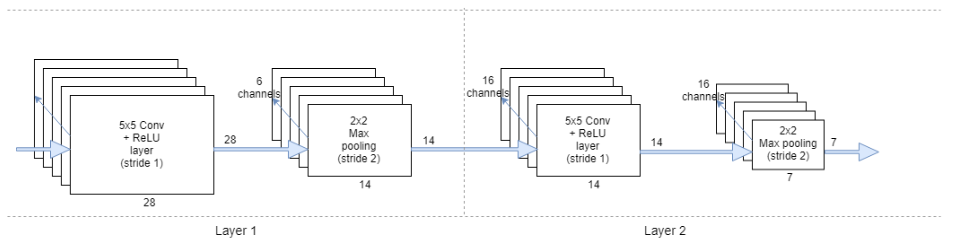Hidden Layers of Convolutional Neural Network

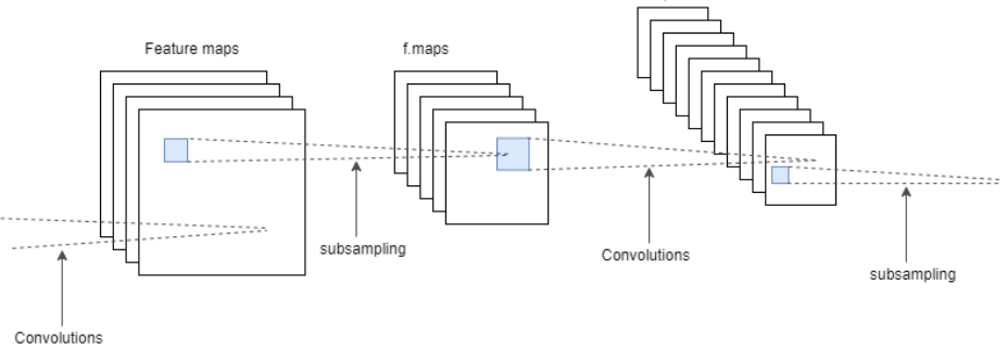Partial Process of Convolutional Neural Network

Implementation

PyTorch

Unlike other frameworks, PyTorch has dynamic execution graphs, and the computation graph is generated instantly. With the imports in place, I set the number of epochs to 10 for preparing the dataset, which indicates that I would loop over the complete training dataset ten times, while learning_rate and momentum are hyperparameters for the optimizer later on. Also, TorchVison handles DataLoaders for the dataset. After loading the MNIST dataset, I use a batch_size of 64 for training and size 200 for testing on this dataset. Below is the structure of my network. I used two 2D convolutional layers followed by two fully-connected layers. As for the activation function, I select rectifier linear units (ReLUs), and then consider torch.nn layers as what will contain the trainable parameters, yet torch.nn.functional are purely functional.

 1
 2
 3
 4
 5
 6
 7
 8
 9
10
11
12
13
14
15
16
17
18
19
20
21
22
23
24
25
26
27
28
29
30
31
32
33

class CNN(nn.Module):
    def __init__(self):
        super(CNN, self).__init__()
        self.conv1 = nn.Sequential(
            # Conv layer 1 output shape (6,28,28)
            nn.Conv2d(1, 6, kernel_size=5, padding=2),
            nn.BatchNorm2d(6),
            nn.ReLU(),
            # Pooling layer 1 (max pooling) output shape (6,14,14)
            nn.MaxPool2d(kernel_size=2, stride=2), 
        )
        self.conv2 = nn.Sequential(
            # Conv layer 2 output shape (16,14,14)
            nn.Conv2d(6, 16, kernel_size=5, padding=2),
            nn.BatchNorm2d(16),
            nn.ReLU(),
            # Pooling layer 2 (max pooling) output shape (16,7,7)
            nn.MaxPool2d(2, 2)     
        )
        self.fc1 = nn.Sequential(
            # Fully connected layer 1 input shape (16*7*7)=(784)
            nn.Linear(16 * 7 * 7, 120),
            nn.ReLU()
        )
        self.fc2 = nn.Linear(120, 10)

    def forward(self, x):
        x = self.conv1(x)
        x = self.conv2(x)
        x = x.view(x.size()[0], -1) 
        x = self.fc1(x)
        x = self.fc2(x)
        return x

TensorFlow

The main concept of TensorFlow is the tensor, a data structure similar to an array. Correspondingly, each epoch in TensorFlow is a full iteration, and I use dropout function in our final hidden layer to give each unit a 50% chance of being eliminated at every training step thus overfitting can be effectively prevented. To build my network, I set up the network as a computational graph to execute with 2 processes. TensorFlow differs from Pytorch because it has two initialization functions named weight_variable and bias_variable. In order to create this model, I need to generate a lot of weights and offsets. The weights in this model should be initialized with a small amount of noise to break the symmetry and avoid the zero gradient. Since I am using ReLU neurons, it is good to initialize the bias term with a small positive number, which avoids the issues of dead neuron.

 1
 2
 3
 4
 5
 6
 7
 8
 9
10
11
12
13
14
15
16
17
18
19
20
21
22
23
24
25
26
27
28
29
30
31
32
33
34
35
36
37
38
39
40
41
42
43
44
45

def weight_variable(shape):
    initial = tf.truncated_normal(shape,stddev = 0.1)
    return tf.Variable(initial)

def bias_variable(shape):
    initial = tf.constant(0.1,shape = shape)
    return tf.Variable(initial)

def conv2d(x,W):
    return tf.nn.conv2d(x, W, strides = [1,1,1,1], padding = 'SAME')

def max_pool_2x2(x):
    return tf.nn.max_pool(x, ksize=[1,2,2,1], strides=[1,2,2,1], padding='SAME')

# Conv layer 1 output shape (6,28,28)
W_conv1 = weight_variable([5, 5, 1, 6])
b_conv1 = bias_variable([6])
x_image = tf.reshape(x,[-1,28,28,1])
h_conv1 = tf.nn.relu(conv2d(x_image,W_conv1) + b_conv1)

# Pooling layer 1 (max pooling) output shape (6,14,14)
h_pool1 = max_pool_2x2(h_conv1)

# Conv layer 2 output shape (16,14,14)
W_conv2 = weight_variable([5, 5, 6, 16])
b_conv2 = bias_variable([16])
h_conv2 = tf.nn.relu(conv2d(h_pool1, W_conv2) + b_conv2)

# Pooling layer 2 (max pooling) output shape (16,7,7)
h_pool2 = max_pool_2x2(h_conv2)

# Fully connected layer 1 input shape (16*7*7)=(784)
W_fc1 = weight_variable([7 * 7 * 16, 120])
b_fc1 = bias_variable([120])
h_pool2_flat = tf.reshape(h_pool2, [-1, 7*7*16])
h_fc1 = tf.nn.relu(tf.matmul(h_pool2_flat, W_fc1) + b_fc1)

keep_prob = tf.placeholder("float")
h_fc1_drop = tf.nn.dropout(h_fc1, keep_prob)

# Fully connected layer 2 to shape (120) for 10 classes
W_fc2 = weight_variable([120, 10])
b_fc2 = bias_variable([10])

y_conv=tf.nn.softmax(tf.matmul(h_fc1_drop, W_fc2) + b_fc2)

Keras

Keras provides a convenient method by having a special layer called flatten layer, which belongs to the core layer. It primarily processes multi-dimensional input as one-dimensional input, which is commonly used in the transition from convolutional layer to fully connected layer. Keras.layers.core.flatten() displays that flatten does not affect the size of the batch. After importing required classes and functions, initializing the random number generator to a constant seed value for reproducibility of results and loading the MNIST dataset, I reshape it in order to be used in training a CNN. It has a similar network as Pytorch and TensorFlow.

 1
 2
 3
 4
 5
 6
 7
 8
 9
10
11
12
13
14
15
16
17
18
19
20
21
22
23
24
25
26
27
28
29
30
31
32
33

model = Sequential()

# Conv layer 1 output shape (6,28,28)
model.add(Conv2D(6, (5, 5),
	padding='same',  
	input_shape=(1,28,28),
	))
model.add(Activation('relu'))
 
# Pooling layer 1 (max pooling) output shape (6,14,14)
model.add(MaxPooling2D(
	pool_size=(2,2),
        strides=(2, 2),
	padding='same',
	))
 
# Conv layer 2 output shape (16,14,14)
model.add(Conv2D(16, (5, 5), padding="same"))
model.add(Activation('relu'))
 
# Pooling layer 2 (max pooling) output shape (16,7,7)
model.add(MaxPooling2D(pool_size=(2,2),padding='same'))
 
 
# Fully connected layer 1 input shape (16*7*7)=(784)
model.add(Dropout(0.2))
model.add(Flatten())
model.add(Dense(120))
model.add(Activation('relu'))
 
# Fully connected layer 2 to shape (120) for 10 classes
model.add(Dense(10))
model.add(Activation('softmax'))